lets learn Pivot Tables in Excel

Pivot tables are among the most useful and powerful features in Excel. We use them in summarizing the data stored in a table. They organize and rearrange statistics (or “pivot”) to draw attention to the valuable facts. You can take an extremely large data set and see the relevant information you need in a clean, concise, manageable way.

Sample Data

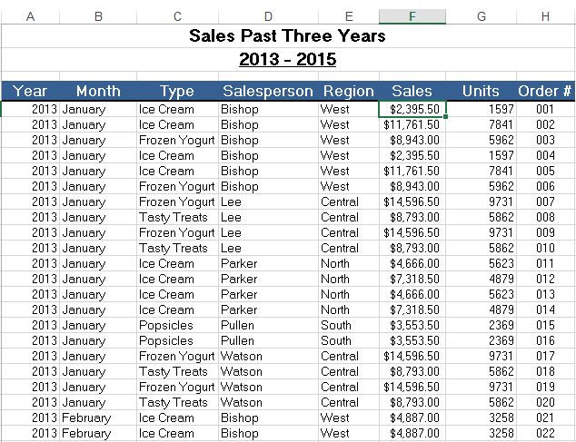
The sample data that we are going to use contains 448 records with 8 fields of information on the sale of products across different regions between 2013-2015. This data is perfect to understand the pivot table.

Insert Pivot Tables

To insert a pivot table in your sheet, follow these steps:

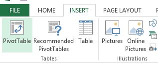
• Click on any cell in a data set.
• On the Insert tab, in the Tables group, click PivotTable.

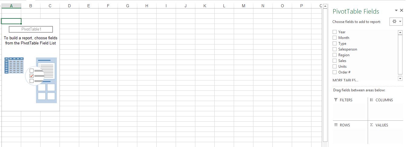
A dialog box will appear. Excel will auto-select your dataset. It will also create a new worksheet for your pivot table.

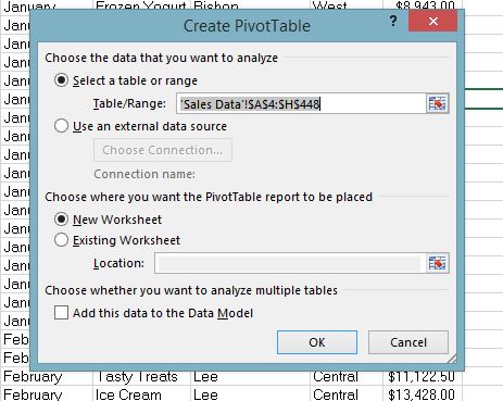
• Click Ok. Then, it will create a pivot table worksheet.

Drag Fields

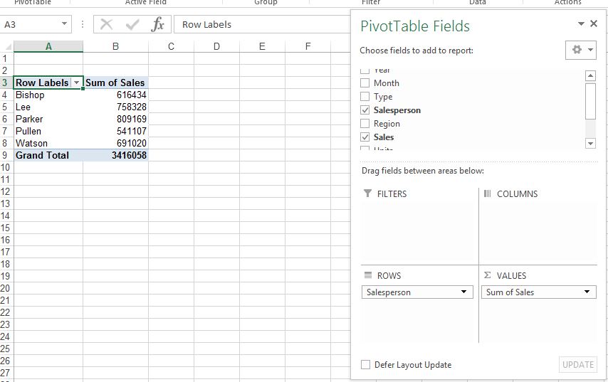
To get the total sales of each salesperson, drag the following fields to the following areas.

• Salesperson field to Rows area.
• Sales field to Values area.

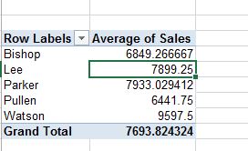
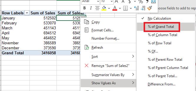
Value Field Settings

By default, Excel gives the summation of the values that are put into the Values section. You can change that from the Value Field Settings. 

• Click on the Sum of Sales in the Values field.

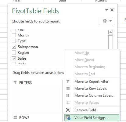
• Choose the type of calculation you want to use.

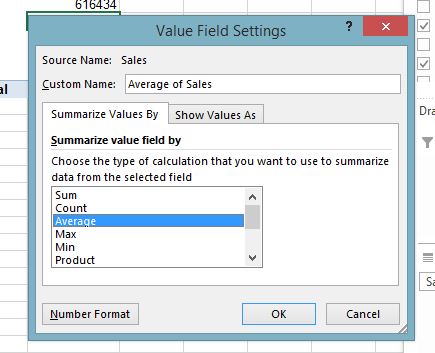
• Click OK.

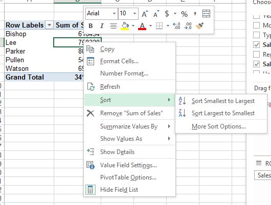
Sorting By Value

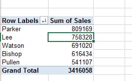
• Right-click any Sales value and choose Sort > Sort Largest to Smallest.

Result:

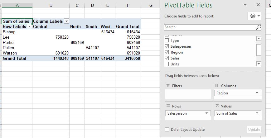
Two-Dimensional Pivot Table

We can create a pivot table in various two-dimensional arrangements. Drag the following fields to the different areas

• Salesperson to Rows area.
• Region to Columns area.
• Sales to Values area.

Applying Filters to a Pivot table

Let’s see how we can add a filter to our pivot table. We will continue with the previous example and add the Year field to the Filters area.

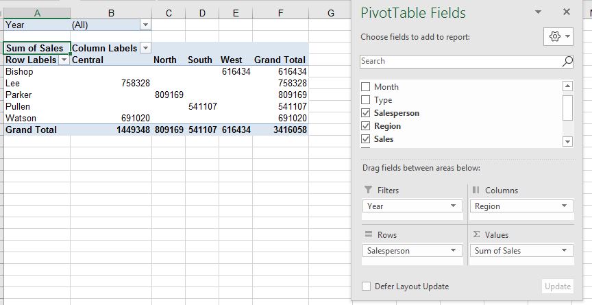
You can see that it adds a filter on the top of the worksheet.

Conclusion

In this article, you’ve learned the basics of pivot table creation in Excel. You can see how simple it is to get started creating one and visualizing your data in many different ways. 

Boost your analytics career with powerful new Microsoft Excel skills by taking the Business Analytics with Excel course, which includes Power BI training

This Business Analytics certification course teaches you the basic concepts of data analysis and statistics to help data-driven decision making. This training introduces you to Power BI and delves into the statistical concepts that will help you devise insights from available data to present your findings using executive-level dashboards.

Do you have any questions for us? Feel free to ask them in this article’s comments section, and our experts will promptly answer them for you!